A trading strategy can win more often than it loses and still lose money. A 70% win rate sounds impressive, but it says nothing about the size of losing trades, trading costs, drawdowns, or how many opportunities produced the result. Win rate is one statistic, not a verdict on strategy quality.
A stronger review combines profitability, loss size, risk, and uncertainty. Expectancy estimates the average outcome per trade. Drawdown shows the depth of losses from a prior account peak. Risk adjusted returns compare gains with the variability or downside risk taken to earn them. Sample size and testing method help show how much confidence the results deserve. Each measure answers a different question, so no single ratio can establish that a strategy will keep working.
Why win rate can mislead
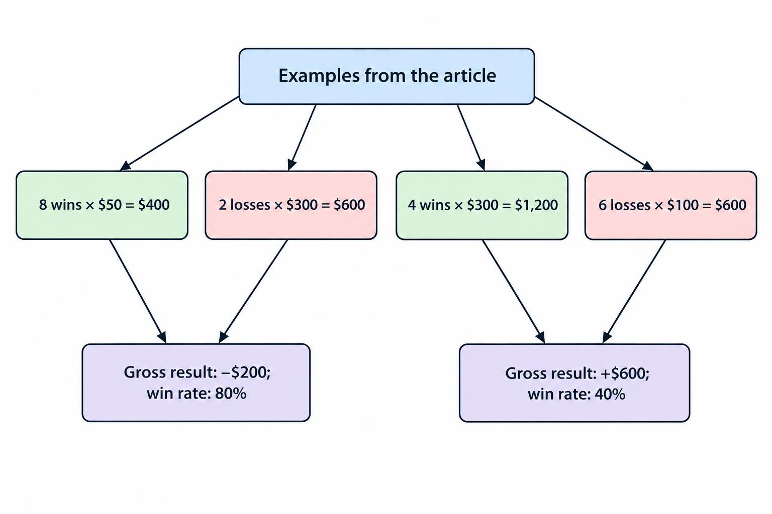
Win rate is the share of completed trades that close with a profit. It is easy to calculate and easy to misread. A strategy might win 8 of 10 trades, earning $50 on each winner but losing $300 on each of the two losing trades. Its gross result is a $200 loss: $400 in wins minus $600 in losses. The 80% win rate does not rescue the arithmetic.
The reverse can happen too. A system may win only 4 of 10 trades but make $300 on each winner and lose $100 on each losing trade. That produces a $200 gross gain. A low win rate is not automatically a bad result if winners are large enough to pay for losses and costs. The relevant question is what the strategy earns or loses across all trades, measured consistently.
Win rate also depends on what counts as a trade, how partial exits are recorded, and whether open positions are included. A strategy can close many small wins while carrying a large unrealized loss, making a closed trade report look healthier than the account’s actual equity. Define the measurement rules before comparing systems.
Start with expectancy
Expectancy estimates the average profit or loss per trade over a defined sample. A simple form is:
Expectancy = (win rate × average win) − (loss rate × average loss)
Use the same unit for average wins and losses, such as dollars per trade, percentage of account equity, or “R,” where 1R is the amount risked on a trade. If 1R equals $100, a winning trade of $200 is +2R and a losing trade of $100 is −1R. R multiples make results easier to compare across position sizes, though they do not replace account level returns or portfolio risk analysis.
Consider a hypothetical strategy with a 45% win rate, an average win of 2R, and an average loss of 1R. Its gross expectancy is (0.45 × 2R) − (0.55 × 1R) = +0.35R per trade. That is a positive average in the sample, not a promise about the next trade. If commissions, spread, slippage, financing, or other costs average 0.4R per trade, the net expectancy becomes −0.05R. The apparent edge has disappeared.
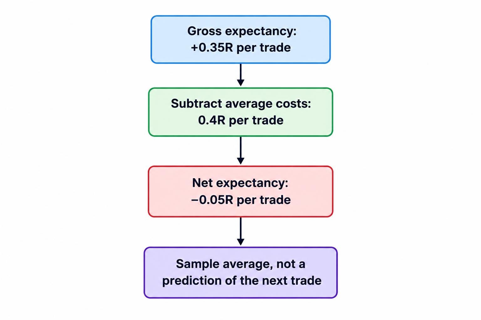
Expectancy should be calculated from realized results after realistic costs. Make sure the numbers use a consistent basis: either all gross or all net, not gross winners paired with losses that include fees. For a practical guide to modelling commissions, spreads, slippage, and financing in tests, see how to include trading costs in backtests.
What expectancy leaves out
A positive average does not tell you how results are distributed. Two strategies can show the same expectancy while one produces frequent small gains and occasional severe losses, and the other produces a steadier sequence. Expectancy also hides the order of trades. A run of losses early in a sample may force a trader to stop before later gains arrive, even when the full-period average is positive.
Break expectancy down by relevant conditions, but avoid treating every subgroup as proof of a separate edge. Results by market, setup, time of day, direction, or volatility can reveal concentration. They can also create a fresh multiple-testing problem if many slices are examined and only the favorable ones are reported. Keep the original sample and criteria visible when reviewing any subgroup.
Measure returns on the account, not only trade outcomes
Per-trade results help explain a strategy, but account-level returns show what an investor might have experienced while positions overlapped, cash remained idle, and position sizes changed. Use a clearly defined equity curve that includes realized and unrealized profit and loss, fees, deposits, withdrawals, and any financing charges that apply. Deposits and withdrawals should not be mistaken for investment performance.
Report the period covered, starting and ending equity, and the return convention used. A simple cumulative return is the percentage change between starting and ending capital after adjusting for external cash flows. Compounded returns account for gains and losses being applied to a changing balance. If comparing strategies, use a consistent time interval and account for differences in leverage, exposure, and cash usage.
Absolute profit on its own is hard to interpret. A $5,000 gain on a $10,000 account is not comparable to the same gain on a $500,000 account, nor does either figure reveal how much risk was taken along the way. Rate of return helps with scale, but it still needs a risk measure and a clear account of costs.
Drawdowns show the path of losses
A drawdown measures the decline in account equity from a prior high. If an account rises to $20,000 and then falls to $16,000, the drawdown from that peak is 20%. The maximum drawdown is the largest peak to subsequent trough decline during the measurement period. It captures a feature that final return can hide: the size of the loss a trader had to endure before the account recovered or the test ended.
Drawdown depends on the sequence of returns. The same set of gains and losses in a different order can produce a different maximum drawdown, even if the total return is identical. For this reason, a report should include a time series of equity or periodic returns, not just a final balance and a drawdown figure.
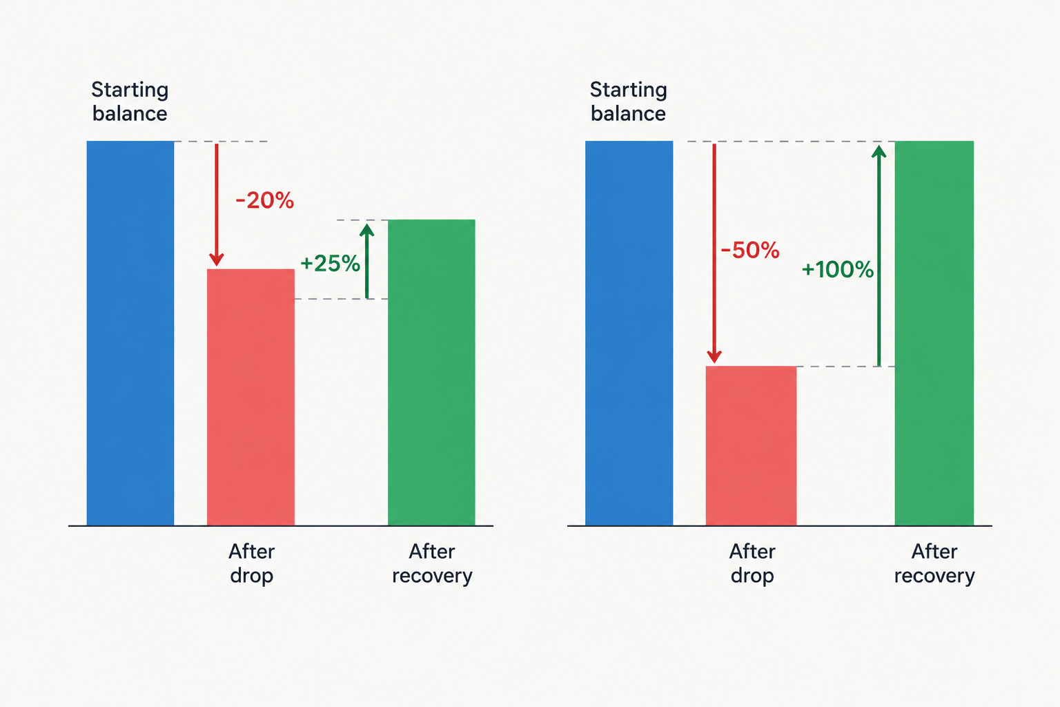
Recovery arithmetic can make a drawdown more tangible. After a 20% loss, an account must gain 25% from its reduced balance to return to the starting level. After a 50% loss, it must gain 100%. The required percentage gain rises as the loss deepens, which is why capital preservation matters even when a strategy’s average return looks attractive.
Maximum drawdown is not the whole risk story
Maximum drawdown is useful, but it describes only the worst observed peak to trough decline in the chosen sample. It does not estimate the worst possible loss, and a longer sample may produce a larger drawdown simply because it includes more opportunities for one to occur. A strategy with a short record and modest maximum drawdown has not proved that severe losses are impossible.
Also record the duration of drawdowns: how long the account stayed below its prior peak, and how long it took to recover, if it did. A 15% decline that lasts several weeks may be harder to manage than a similar decline that lasts years. The practical impact depends on the trader’s funding, obligations, strategy rules, and ability to continue following the system.
Look at both percentage drawdown and dollar loss. A 10% decline means different amounts of money in different account sizes, while a dollar figure alone does not show the loss relative to capital. If a model uses leverage, include the exposure and margin assumptions behind the equity curve; a smooth percentage return can conceal a position size that would be difficult to maintain through adverse moves.
Risk adjusted returns: what the ratios say
Risk adjusted measures relate returns to a chosen definition of risk. They are useful for comparison, but each ratio compresses a complex return history into a single number. Check the inputs, period, and calculation method before comparing reported values.
| Measure | What it compares | What to watch |
|---|---|---|
| Sharpe ratio | Average excess return relative to the standard deviation of returns | Can be affected by outliers, short samples, non-normal returns, and serial correlation |
| Sortino ratio | Return relative to downside deviation, using a stated target or minimum acceptable return | The downside threshold and calculation method must be disclosed |
| Calmar ratio | Annualized return relative to maximum drawdown over a stated period | Highly sensitive to the sample’s single worst drawdown and the period selected |
| Profit factor | Gross profits divided by gross losses | Does not account for capital tied up, return volatility, or the sequence of losses |
Sharpe ratio
The Sharpe ratio compares average return above a chosen risk free rate with the standard deviation of returns. In a common periodic form, it is the mean excess return divided by the standard deviation of excess returns. Annualized figures often scale a periodic ratio by the square root of the number of periods in a year, an approximation that can mislead when returns are serially correlated or the data do not fit the calculation’s assumptions.
Sharpe is not a complete measure of risk. Standard deviation counts upside and downside variability, so a large positive return can increase the measured volatility even when an investor would welcome the gain. More seriously, a high estimated Sharpe from a short or heavily selected backtest may be a product of noise. Bailey and López de Prado’s research on the Deflated Sharpe Ratio addresses sample length, non-normal returns, and selection bias from testing multiple strategies. The broader lesson is simple: a ratio selected from dozens or hundreds of experiments needs more scrutiny than a result specified in advance.
Sortino and Calmar ratios
The Sortino ratio replaces total return variability with downside deviation relative to a stated target, such as zero return or a minimum acceptable return. That can make it more relevant when downside swings matter more than upside variation. But the chosen target changes the result, and downside deviation still depends on the period and data used. A Sortino number without its target is incomplete.
The Calmar ratio commonly compares annualized return with maximum drawdown over a specified period. It is intuitive because it puts a return figure beside the worst historical peak to trough loss. Yet it can swing sharply when the sample’s worst drawdown changes, and it says little about the frequency or duration of losses. Treat it as one view of the equity curve, not a score that settles the comparison.
Profit factor, the ratio of gross winning dollars to gross losing dollars, can help describe whether gains exceed losses in aggregate. A value above 1 means gross profits exceeded gross losses in the measured sample; it does not mean the strategy is profitable after all costs. It also gives no direct account of capital requirements, idle periods, position overlap, or how many trades generated the result.
Compare like with like
A comparison is only useful when the strategies face similar measurement rules. Align the market, time period, data frequency, account size assumptions, order timing, and cost model. Include the same spread and slippage assumptions where relevant. If one strategy trades frequently and another rarely, report both per trade and per time period, and disclose how capital is allocated between them.
Compare a strategy with a relevant simple rule or benchmark, not only with other complex systems. A model may produce positive returns but still add little value if a simpler approach delivered a stronger return for similar risk, or if the model’s extra costs erase its advantage. Choose the comparison before reviewing the final test results. The guide to comparing a strategy with simple rules and relevant benchmarks covers that choice.
Do not compare a hypothetical backtest with live results as if they were equivalent evidence. Backtests depend on assumptions about data, fills, costs, and trade execution; live records include real order handling and the pressures of actual losses. The CFTC’s advisory on commodity trading systems warns that hypothetical results may not reflect actual trading conditions, including spreads, execution prices, market impact, and the trader’s capacity to sustain losses. Those points are relevant whenever a performance claim relies on simulated trades.
Sample uncertainty and the danger of a lucky result
Every performance statistic is estimated from a sample. A result based on 20 trades can change sharply when a few trades are added or removed. A result based on several hundred trades can still be unreliable if the trades are highly dependent, drawn from one unusual market period, or selected after repeated strategy tweaking. Trade count is not the same thing as independent evidence.
Look at the number of trades, the length of the record, and the range of market conditions represented. A strategy tested during a strong trend may behave differently in a choppy market; a short record may not include a rare but damaging event. Neither a long calendar period nor a high trade count guarantees that the sample represents the next period.
Multiple testing is another source of overconfidence. If a researcher tries many indicators, parameters, assets, and exit rules, then reports only the best performer, some of its apparent edge may come from chance. Keep a record of the trials, avoid using the same data repeatedly to select and confirm a model, and reserve untouched data for final evaluation. For a fuller treatment, see how overfitting and data leakage distort trading tests.
Use time ordered validation rather than randomly mixing future and past observations. A clean test period should remain separate from model selection; walk forward evaluation can then examine how a fixed process behaves as new periods arrive. These methods reduce some forms of leakage and selection bias, but they do not eliminate uncertainty or guarantee future performance. See how to split financial time series for training and testing and how walk forward testing evaluates a strategy through time.
Practical checklist for reviewing a strategy
A sound performance review puts multiple views side by side. The aim is not to find one perfect score, but to check whether the reported edge survives reasonable changes in measurement and conditions.
- Net expectancy: Calculate the average outcome after realistic commissions, spread, slippage, financing, and other costs.
- Return: Show account level returns over a stated period, with deposits and withdrawals treated separately.
- Drawdown: Report maximum percentage drawdown, dollar loss, duration, and recovery status.
- Risk adjusted measures: Include a suitable ratio, disclose its inputs, and do not rank strategies using one ratio alone.
- Sample: State the number of trades, date range, markets, and conditions represented.
- Selection history: Record how many versions, parameters, or alternatives were tested before choosing the reported result.
- Evidence type: Label results as live, paper, or backtested, and state the assumptions used to produce them.
Then inspect the equity curve and the distribution of trade outcomes. Check whether a small number of exceptional winners account for most of the profits, whether losses cluster in a particular condition, and whether a modest change in costs removes the apparent edge. A strategy whose return depends on one lucky trade, an unrealistic fill, or a favorable market regime deserves a lower level of confidence.
Paper trading can test whether alerts, order logic, and operational assumptions behave as intended, though it cannot fully reproduce financial risk or live execution. A paper record is a different evidence category from a backtest or funded trading history. The article on what paper trading can establish explains what simulation can and cannot confirm.
How to interpret a performance claim
When reviewing a published result, ask whether the reported win rate is supported by average win and average loss, and whether costs are included. Find out whether returns are gross or net, what capital base was used, and how maximum drawdown was calculated. Check whether the results came from actual trading or a simulation, and whether the strategy was chosen after testing many alternatives.
Be cautious with impressive ratios that have no period, sample size, benchmark, or calculation method attached. A single headline statistic cannot show whether a strategy is robust, scalable, or tolerable for a particular trader. The CFTC also notes that past results do not predict future results, and distinguishes actual account performance from hypothetical or simulated records in its guidance for commodity trading disclosures. That is a reminder to treat a performance record as evidence about the period tested, not a forecast.
Win rate belongs in a trading report because it describes how often trades were profitable. It should sit beside expectancy, net returns, drawdown, risk adjusted measures, and sample details. When those figures point in different directions, investigate why. That tension often reveals more than the win rate alone.