Feature selection decides what information a trading model can use before it estimates a signal. That choice affects what the model learns, how it behaves when market conditions change, and whether a backtest reflects information that was actually available at the time. Adding more inputs is easy. Finding inputs that provide useful, timely information without duplicating one another is harder.
A sound feature set begins with a clear prediction target and decision time. A model forecasting the next session’s return needs different inputs from one estimating volatility over the next month. A feature can look predictive in historical data yet be unusable if it depends on a value published later, or if its apparent contribution disappears after trading costs. The practical goal is not to collect every indicator. It is to test a small, defensible set of inputs against a defined task and retain only those that improve results outside the data used to choose them.
Start with the prediction target
Features are inputs; the target is what the model is asked to estimate. That may be a future return, the probability of a positive return, a volatility estimate, or a market condition such as a trend or range. Decide the target’s horizon and the moment when the model is supposed to act before selecting features. Otherwise, a feature may be measured over the wrong window, or its calculation may accidentally include information from the period being predicted. The distinctions between predicting prices, returns, direction and probabilities matter because each choice changes how model output should be read.
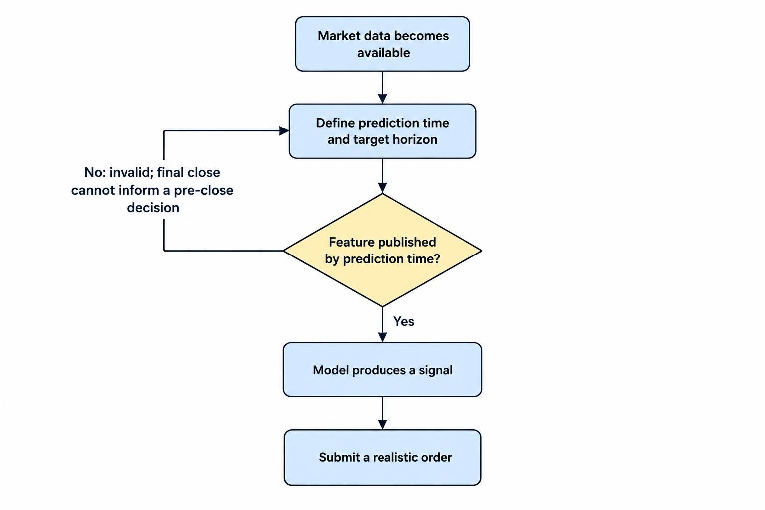
Write down the decision schedule in plain language: what data is known, when the prediction is made, and when an order could realistically be submitted. For example, a model that uses a day’s closing price cannot use that final value to make a decision before the close. A signal computed after the close may be valid for a later order, subject to the execution assumptions in the test. This timing rule applies to every input, including data that appears harmless, such as a rolling average or a calendar field. The model cannot know more than the trader could have known at that point.
Price features: use changes and relative levels
Raw prices often make poor inputs across different securities or time periods. A share trading at $20 and one trading at $200 are not directly comparable just because their prices differ by a factor of ten. Price levels can also rise over time, leaving a model to learn scale or trend effects that do not transfer. Returns, percentage changes, and log returns express movement relative to the starting value. They are common starting points for return forecasts, though they do not guarantee that the series is stable or predictable.
Other price-derived features describe the recent path. A return over several sessions can represent momentum; a short return compared with a longer one can describe recent acceleration or reversal. Distance from a moving average can express how far price has moved from a recent reference point. A position within the recent high-to-low range describes where the latest price sits relative to that window. Each calculation needs a defined lookback period, and the period should match the trading question rather than be chosen because it makes an attractive backtest.
Related indicators can carry almost the same information. A moving-average crossover, a difference between short- and long-window returns, and a price-to-average ratio may all reflect recent direction. Giving the model all three does not necessarily provide three independent clues. Start with a small number of interpretable price features, then compare the added value of related candidates. If the goal is to screen trend setups, focus on a few measures of direction, persistence and distance from a reference level. The guide to filtering trend-following signals covers that use case in more detail.
Volume features: measure activity, not just size
Volume can add information about trading activity, but raw volume is tied to the instrument, its price, and its usual level of activity. A more comparable input might measure current volume against its own recent average, or express turnover relative to the amount normally traded. A change in activity can help describe whether a price move is occurring alongside unusually high or low participation. That is a candidate signal to test, not a rule that high volume confirms a trade.
Data quality matters. The meaning and completeness of volume vary by market and data provider, while some markets report only part of total activity. If the model covers several instruments, confirm that the volume values are comparable and that adjustments for splits or contract changes are handled consistently. For intraday strategies, time of day also matters: a reading can be unusual compared with the prior hour but normal for the same time on another session. Features should be calculated from data available at the prediction time, and the same data rules should apply in training, testing and live use.
Volatility features: describe the size of recent moves
Volatility features describe how much prices have been moving, rather than whether they will rise or fall. Common candidates include rolling standard deviations of returns, ranges based on high and low prices, and changes in those measures over time. A model might use them to estimate the likely scale of future moves, adjust a signal threshold, or distinguish calmer periods from more volatile ones. If the task is to predict returns, volatility may serve as context rather than a directional forecast.
Lookback length changes the meaning of a volatility measure. A short window reacts quickly but can be dominated by a small number of large moves; a longer window is smoother but can lag a sudden shift. Compare windows chosen for a practical reason, not dozens of arbitrary settings. Where appropriate, express volatility relative to the instrument’s own history, using only observations available at the time. A full-sample average or maximum used to normalize earlier observations can quietly insert future information into the feature.
Volatility can also change the economics of a signal. A model that appears useful on average may trade too often or take too much risk during turbulent periods. Consider whether volatility should enter the model, inform position sizing, or be used as a condition for allowing a trade at all. Those are separate design choices; combining them without testing makes it harder to tell which part is doing useful work. A market regime model can provide a fuller treatment of changes between trends, ranges and volatility conditions.
Context features: add only information available at decision time
Context features describe conditions around the instrument: the broader market’s return, a related asset’s movement, a trading-session marker, or a known calendar event. They can help a model distinguish an individual move from a wider market shift. In a stock model, for example, the same return may carry different meaning when the benchmark is rising sharply than when it is falling. Whether that distinction improves a forecast depends on the target, sample and method. A large empirical asset-pricing study found that momentum, liquidity and volatility measures featured among dominant predictive signals in its setting, but that result does not establish a universal recipe for short-term retail trading. The NBER study of machine learning in empirical asset pricing describes its research design and findings.
Calendar and event information needs careful timing. A scheduled event may be known in advance, but the reported result is not available until its release. Company fundamentals should be dated by public availability, not simply assigned to the accounting period they describe. News features need the same discipline: record when the article or update became available, and do not treat a later revision as if it were present earlier. When a feature comes from another market or instrument, check its trading hours and publication schedule against the model’s decision time.
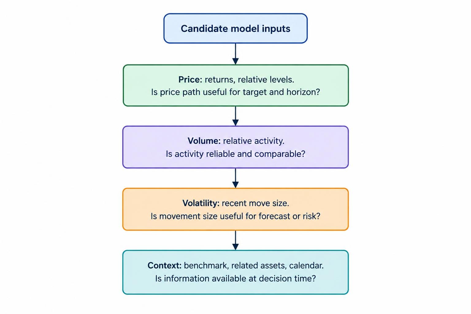
| Feature family | Possible inputs | Question to test |
|---|---|---|
| Price | Returns, distances from rolling averages, position within a recent range | Does the recent price path add information for this target and horizon? |
| Volume | Relative volume, turnover, change in activity | Is the activity measure reliable and comparable for this instrument? |
| Volatility | Rolling return variation, high-low range, change in volatility | Does recent movement size help forecast the target or manage the signal? |
| Context | Benchmark returns, related assets, session or scheduled-event markers | Was the information available when the model would have acted? |
Transform features to fit the decision
A model may need inputs in a scale that makes comparisons useful. Returns are already expressed as relative changes, while price distances can be divided by a recent price or volatility estimate. Volume might be compared with a rolling baseline. Scaling is a modelling choice, not a way to make a weak input meaningful. The rule used to calculate a transformation must be learned from the training data and applied consistently to later data. If the test period influences the mean, standard deviation, minimum or maximum used for scaling, the evaluation is no longer a clean simulation.
Lookback periods and lags need equally clear definitions. A five-session return uses a different information window from a twenty-session return; a lagged feature may be appropriate when the most recent value is unavailable at order time. Rolling calculations also need a warm-up rule for their first observations. Avoid filling missing values with a number that carries an accidental meaning, and check that the same missing-data policy could be used in live operation. Preparing historical market data for model research is part of feature design, not a separate cleanup step to leave until later.
How to select features without selecting noise
Feature selection methods usually fall into three broad groups. Filter methods rank inputs using a measure such as correlation with the target, then remove or retain them before fitting a model. Wrapper methods compare candidate sets by repeatedly training a model and measuring its performance. Embedded methods select or down-weight inputs as part of training, as some regularized models do. Each method answers a slightly different question. A high correlation with a target does not prove a feature will improve a trading strategy, while a feature that matters inside one model may not matter in another.
Start with a reason for each candidate: what information does it represent, and why might that information matter to the target? Then use a modest set of candidates, including simple reference features, and evaluate them with chronological splits. Feature selection belongs inside the training process for each split. Selecting inputs once using the full history and then reporting test performance leaks knowledge from the future into the model-building decision. The paper on information leakage in financial machine learning discusses this problem, including leakage from full-sample feature selection and preprocessing.
Correlated inputs complicate interpretation. If two features carry similar information, one may receive a high importance score while the other receives little, even though removing either one alone barely changes predictions. Conversely, a feature may appear important because it tracks a market condition that the model could represent through another input. Check groups of related features, not just a ranked list of individual scores. Importance estimates help describe how a fitted model uses inputs; they do not show that a feature causes returns or will remain useful in another period.
Repeated testing creates another trap. If many features, lookbacks, model settings and rules are tried against the same history, the best result may be the luckiest combination rather than a durable signal. Keep a record of the alternatives tested, preserve a final holdout period, and avoid using that holdout to guide further changes. Researchers have proposed methods for assessing how often an in-sample winner ranks poorly out of sample; the study defining probability of backtest overfitting describes one such framework. It is a diagnostic, not a substitute for sound data and test design.
A practical feature-selection workflow
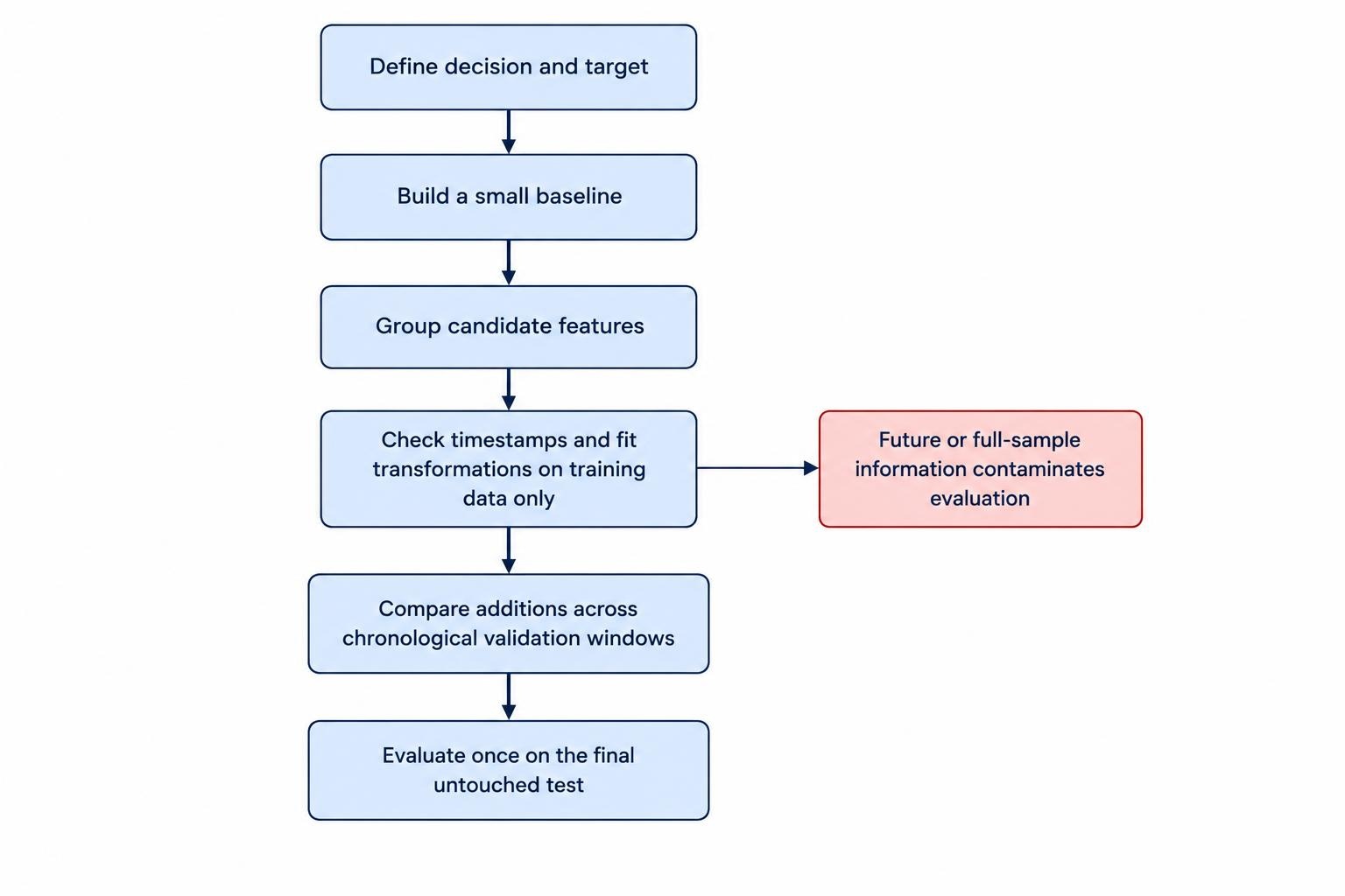
- Define the decision. Specify the instrument universe, forecast target, horizon, prediction time and earliest realistic execution time.
- Build a small baseline. Use a few straightforward inputs, such as lagged returns and a volatility measure. Record performance before adding complexity.
- Group candidates by information. Separate price path, activity, volatility and context. This makes overlap easier to spot and gives each addition a clear purpose.
- Check timestamps and transformations. Confirm that inputs were available at the decision time, and fit preprocessing rules using only each training window.
- Compare additions out of sample. Add one feature or coherent feature group at a time. Compare results across chronological validation windows, not just one favourable period.
- Retain a final untouched test. Do not repeatedly inspect the holdout and revise the feature set in response. Once that happens, it has become part of development.
These steps depend on a valid testing design. Training, validation and test periods should respect time order, and any label whose future return window overlaps a split boundary may require special handling. See the guide to splitting financial time series into training, validation and test sets for the mechanics. When features or labels overlap across adjacent observations, an ordinary random split can make evaluation look cleaner than a real forecasting process would be.
Judge feature sets by the results that matter to the intended strategy. Forecast error or classification accuracy can help assess a model, but they do not show whether a trading rule survives fees, spreads, slippage and execution limits. Compare the model against a simpler rule and a relevant benchmark, then examine performance across test periods rather than relying on a single aggregate score. The guides to comparing a strategy with simple rules and benchmarks and including trading costs in backtests cover those checks.
Keep the feature set useful and maintainable
A feature that improves one historical test may be fragile, hard to source consistently, or costly to calculate at the required frequency. Before retaining it, check whether its value persists across different test windows, whether a simpler substitute performs similarly, and whether its data feed can be maintained. If removing it barely changes out-of-sample results, the simpler model may be easier to monitor and less exposed to data problems. More inputs also mean more choices during development, which increases the chance of finding a flattering result by repeated experimentation.
Record each feature’s definition, source, timestamp rule, lookback period, transformation and reason for inclusion. Recheck the set when data quality changes or performance shifts, but do not add or remove features merely because a recent stretch looks uncomfortable. Track proposed changes as new experiments and test them with a fresh evaluation plan. A consistent walk-forward evaluation can show whether a feature set continues to help as the model is retrained through successive periods. The aim is a compact set of inputs that improves the defined decision under realistic tests, not a collection of indicators that explains the past after the fact.