Mean reversion is the idea that an unusually large move away from a reference level may partly reverse. In trading, that reference might be a recent average, a relationship between two assets, or a modelled equilibrium. The signal is not a promise that price will turn. A market can keep moving away from its recent range, and a relationship that once held can break. An AI model can help rank potential setups or estimate the chance of a reversion over a chosen period, but it cannot make the market revert.
A practical system therefore needs two answers: what counts as an unusual deviation, and what evidence would show that the setup has stopped working? Those questions belong at the center of AI trading strategy development. The model’s job is to assess a defined setup under defined conditions, not to label every sharp drop a bargain or every rally an overreaction.
What a mean reversion setup measures
A basic mean reversion signal measures distance from a reference level. One common approach is to calculate a standardized score, often called a z score: the current deviation from the reference divided by an estimate of recent variability. A high positive score means the value sits unusually far above the reference; a high negative score means it sits unusually far below. The score describes distance, not direction with certainty. It also depends on choices such as the lookback period, the reference level and the volatility estimate, so it can change substantially when those choices change.
The reference itself matters. A moving average can describe recent price behavior, but a market trending strongly may stay on one side of it for a long time. A pair or spread strategy instead tracks the difference between related instruments, sometimes after adjusting for their relative movement. A broad market move, an earnings announcement or a change in an instrument’s fundamentals can disrupt that relationship. Research on pairs trading models notes that uncertainty in the estimated long-term mean and volatility can undermine assumptions of reliable arbitrage. A statistical relationship is a working hypothesis, not a guarantee of convergence. Research on parameter uncertainty in pairs trading discusses this limitation.
Before training a model, specify the object being measured. Is it an asset’s price deviation from a rolling average, a spread between two assets, or a return relative to a market or sector? State how the reference is calculated, what data is available at the decision time, and how long the forecast remains relevant. These details stop a model from quietly switching between different meanings of “reversion.” They also make it possible to compare results across instruments and periods without mistaking a change in measurement for a change in market behavior.
How AI can filter a candidate setup
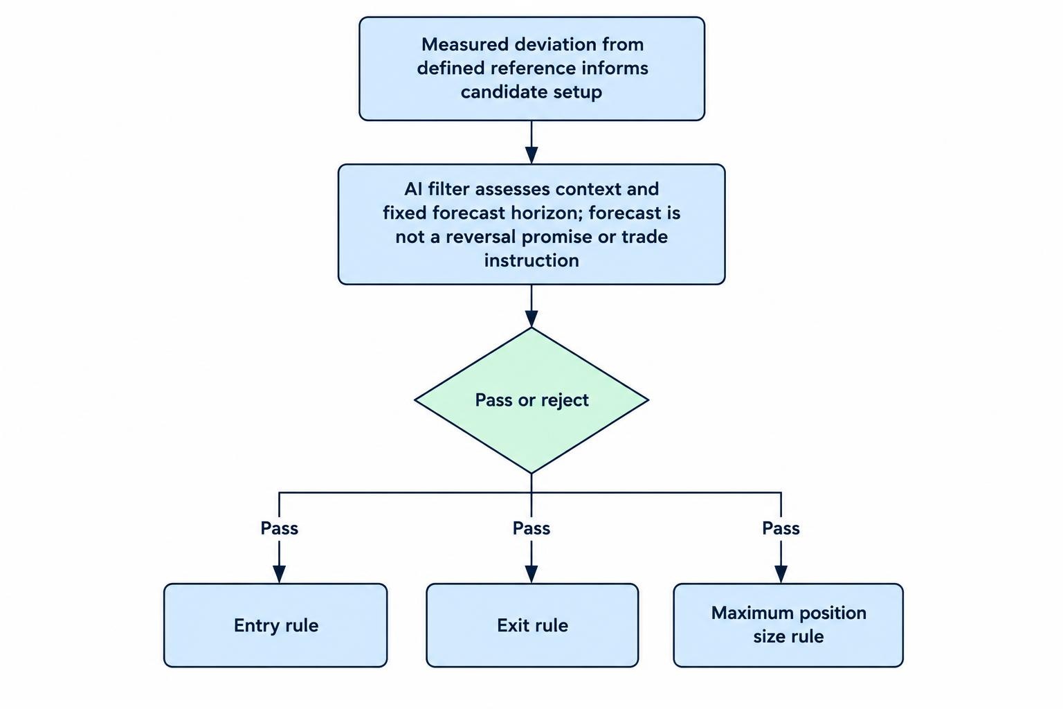
A simple rule can flag a setup whenever a deviation passes a chosen threshold. An AI model can add context: given the size of the deviation and information available now, how often did similar conditions lead to a partial reversal within a fixed horizon? That is a narrower and more testable question than asking a model to predict the next price. The output might be a probability, a ranking score or a decision to pass. A model that returns a high probability still needs a clear definition of what counts as a successful reversal, and what happens if the price keeps moving against the position.
Useful inputs may include the size and direction of the deviation, recent volatility, trading volume, time of day, and the behavior of a relevant index or related instrument. The right inputs depend on the setup. A pair strategy may need the spread’s recent behavior and a way to track the relationship between the two instruments; a single-asset strategy may rely more on price, volume and market context. The model should only use information that would have been available when the simulated decision was made. A guide to choosing features for a trading model can help organize those inputs without turning the data set into a grab bag of indicators.
Define the prediction target just as carefully. “Price will go up” is not the same as “price will move closer to its reference level within ten sessions.” The second statement identifies both a direction and a time limit, but it still needs a rule for measuring the move and handling trades that never reach the target. A useful model may estimate the chance of reaching a reversion level before a risk limit, or the expected return after costs over a stated horizon. The article on choosing prediction targets for trading models covers how target definitions shape what a model learns.
AI does not have to make the final trade decision. A filter can pass only setups that meet a minimum evidence threshold, while a separate rule sets the entry, exit and maximum position size. This keeps the forecast and the trade mechanics distinct. It also makes errors easier to diagnose: a weak forecast, a badly chosen threshold and poor execution are different problems. If the model’s output is difficult to explain in terms of the inputs it receives, the system should be treated as harder to inspect, not automatically more capable.
Illustrative example: a spread moves away from its reference
Suppose two related instruments have usually moved in a reasonably stable relationship. A trader calculates their spread using a hedge ratio estimated from past observations. The spread then moves far above its recent reference. That move creates a candidate setup; it does not prove the spread is “too high.” A model could estimate whether comparable deviations, under similar volatility and market conditions, tended to narrow over the next several sessions. A backtest would then test the forecast using only information available at each decision point, and would account for the position in both instruments.
For a simple illustration, assume the spread is three recent standard deviations above its reference. That figure is not a recommended entry threshold. It is a way to describe an unusually large deviation relative to the chosen sample. If the model estimates a stronger chance of narrowing when volatility is moderate and the relationship has remained stable, it might rank the setup above one occurring during a market shock. The signal could still fail: one instrument may react to new information, the hedge ratio may no longer fit, or the spread may continue widening before any reversal occurs.
In a single-asset setup, the same logic applies to a price that has moved unusually far from a rolling reference. The model can compare conditions with historical cases and estimate the chance or scale of a partial return within the chosen horizon. But a recent average is not an intrinsic value. A company’s price may shift after an earnings surprise, and a currency may move as interest-rate expectations change. The reference can lag behind a genuine repricing. The model should be allowed to reject a candidate when the context no longer resembles conditions under which the signal was tested.
Failure conditions to define before a trade
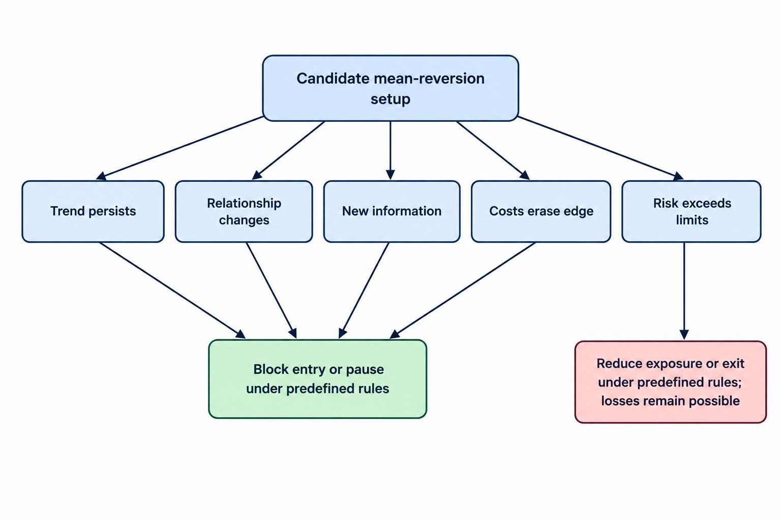
A trend persists. A large deviation can be the early stage of a sustained move rather than a temporary overshoot. Mean reversion is especially vulnerable when the market’s direction or volatility changes. A model can use trend and volatility measures as context, but those measures should be defined before testing. They should not be added one by one until a historical chart looks tidy. A separate market regime detection guide covers ways to distinguish trend, range and volatility conditions.
The relationship changes. For a spread, a historical connection between instruments may weaken after a business change, policy shift, index rebalance or other event. A fitted hedge ratio can become stale. The signal may then be trading an old relationship rather than a temporary gap. Define how the system detects deterioration and what it does next: reduce exposure, stop opening positions, or recalculate the relationship using a pre-specified process. Re-estimating parameters every time a trade looks uncomfortable can hide failure rather than solve it.
The move reflects new information. An abrupt price change may follow an announcement or a change in expectations. A model based on ordinary fluctuations may not handle those events well, especially if its historical sample contains few comparable cases. News and event data may be incomplete, delayed or difficult to interpret consistently. A practical system can exclude defined event windows, reduce exposure, or require a separate review; it should not assume that an AI-generated summary establishes why the price moved.
Costs erase the edge. Mean reversion signals can generate frequent entries and exits. Spreads, commissions, slippage, financing and, where relevant, borrow costs reduce the return available to the trader. A signal that looks profitable before these costs may not survive realistic execution assumptions. Estimate costs in the same units and at the same trade frequency as the strategy, then stress them above the baseline. See how to include trading costs in AI backtests.
The risk is larger than the forecast suggests. A high probability of a small reversion does not rule out a larger loss when the forecast is wrong. Several positions may also depend on the same market factor, even when they involve different instruments. Define maximum exposure, a position exit rule and a portfolio-level loss limit before deployment. A model’s score should not override those limits, and a stop order should not be treated as a guarantee of the eventual fill price in fast markets.
How to test a mean reversion model fairly
Start with a transparent baseline, such as a fixed deviation threshold with pre-defined entry and exit rules. Then compare the AI filter against that baseline and against a relevant benchmark. If the model only looks better than doing nothing, it may be exploiting broad market behavior rather than adding value to the setup. Record how many model versions, feature sets and thresholds were tested. Searching many alternatives on the same historical data makes it easier to select a lucky result. Research on the probability of backtest overfitting describes why a strong in-sample result can fail to hold up on new data.
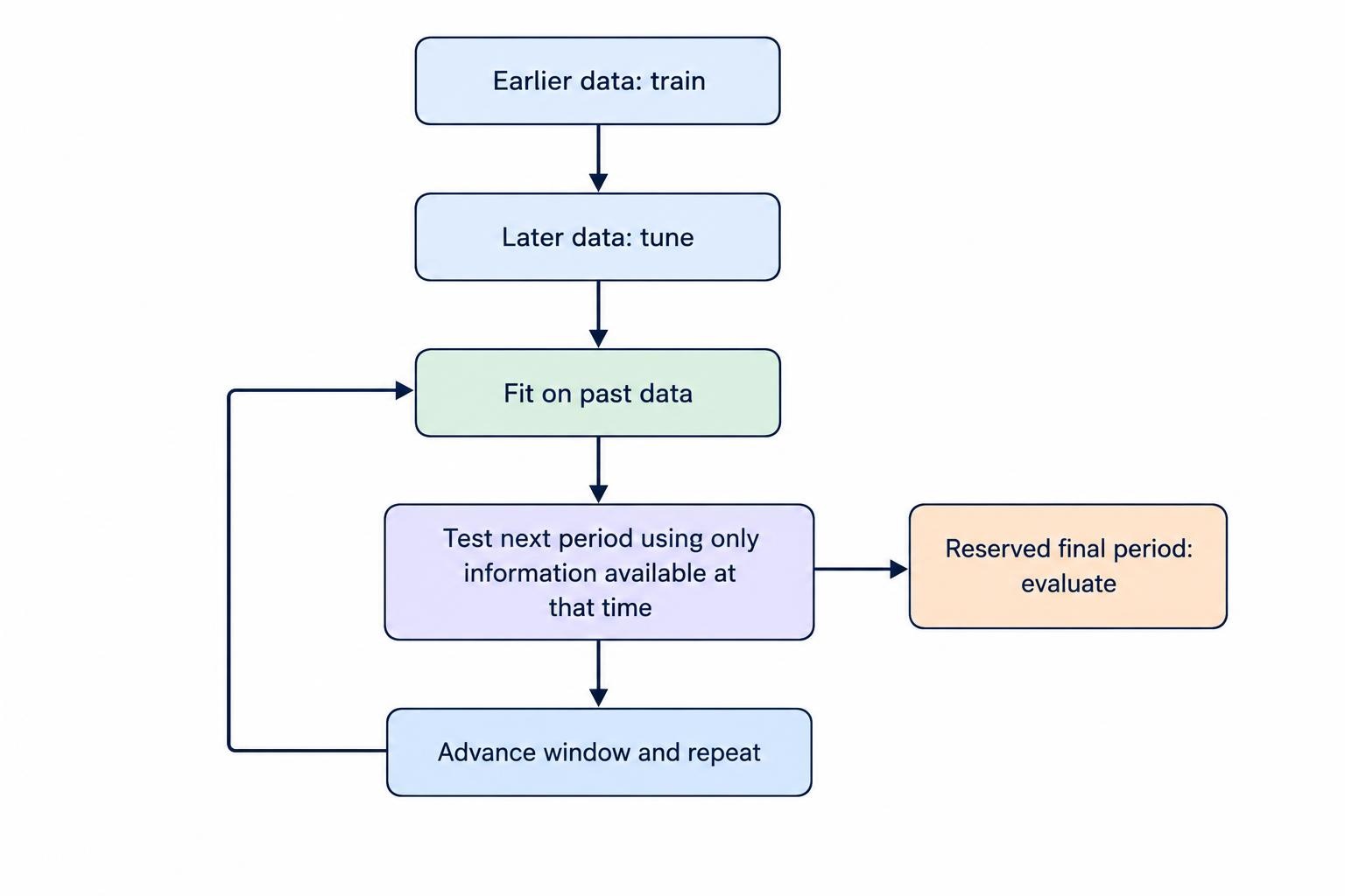
Use chronological data splits. Train on an earlier period, tune using a later period, then reserve a final period for evaluation. Do not randomly shuffle observations from a time series in a way that lets future market conditions inform the past. In rolling or expanding tests, each simulated decision should use parameters estimated only from data available by that point. The guide to splitting financial time series into training, validation and test sets explains the role of each segment, while overfitting and data leakage in trading models covers common ways future information slips into a test.
Use walk-forward testing to see how the strategy behaves as time advances: fit the model on past data, test it on the next period, then move forward and repeat. Keep the rules for updating the model fixed in advance. A model that needs frequent redesign to retain its historical performance may not have a stable signal. Inspect results across different market periods, instruments and levels of trading activity rather than relying on one headline metric. The walk-forward testing guide sets out this process.
Measure more than win rate. A high proportion of small gains can sit beside occasional large losses, and an average return can conceal long flat periods or sharp drawdowns. Review net returns after estimated costs, drawdowns, exposure, turnover and the distribution of trade outcomes. Compare the AI filter with the simple rule under the same assumptions and data. Performance metrics beyond win rate can help keep that assessment grounded.
Set rules for live or simulated use
Before running a model, write down the conditions that create a candidate, the conditions that block it, and the evidence that would trigger a pause. For example, a system might stop opening positions if the spread’s behavior shifts outside the tested range, if the required data becomes stale, or if execution costs rise beyond the level used in the test. These are operational safeguards, not proof that losses cannot occur. They make it clearer when the model is operating outside its research assumptions, and give a trader a reason to investigate instead of rationalizing a bad run.
Paper trading can reveal timing, data and workflow problems, but simulated fills may differ from live fills, particularly when liquidity is thin or prices move quickly. Record the forecast, reference level, proposed position, actual simulated fill and reason for exit. Compare those records with the model’s original assumptions. The paper trading guide explains what simulated results can and cannot establish. Keep the model’s scope modest until its behavior has been checked under conditions it did not help define.
A sound AI-assisted mean reversion system treats every setup as a conditional hypothesis: the deviation is unusual, the historical relationship may still apply, and the expected movement could exceed the cost and risk of taking a position. The model can help rank those hypotheses. The evidence must show whether the filter adds value beyond a simple rule, whether that value survives realistic costs, and where the setup should be rejected.