A trading model can produce an impressive historical result for the wrong reason. It may have been tuned to quirks in the sample, allowed to use information that arrived after a trade decision, or tested on data that was cleaned or revised with future knowledge. These problems often appear together, but they are not the same. Overfitting means a model or strategy has adapted too closely to the data used to develop it. Look-ahead bias means a test uses information that would not have been available at the time of a simulated decision. Data leakage is the broader failure that lets information from outside a model’s legitimate training process affect its inputs, fitting, selection or evaluation.
The distinctions matter because each problem needs a different check. A chronological split can reduce one kind of look-ahead, but it cannot undo a feature built from revised data. A clean point-in-time dataset cannot stop a researcher from trying hundreds of variants and reporting only the winner. And a strong test score cannot reveal a leak if the same contaminated process was used to make and check the predictions. A reliable review therefore follows the full chain: what was knowable, when it was knowable, what was fitted, which choices were tried, and which data were kept untouched until the end.
How the three problems differ
| Problem | What goes wrong | Typical example | First line of defence |
|---|---|---|---|
| Overfitting | A model or strategy learns noise or sample-specific quirks rather than a repeatable pattern. | Trying many indicator settings and keeping the one with the highest backtested return. | Track every trial; reserve later data for evaluation; test stability. |
| Look-ahead bias | A historical decision is made using information that arrived later. | Using a company’s final quarterly earnings figure before that figure was released. | Timestamp each input and align it to the first time it was available. |
| Data leakage | Information crosses a boundary where it should not: from future observations, target construction, test data or later processing. | Scaling all observations before a time split, so test-period statistics affect the training features. | Fit every learned transformation on training data only; audit the pipeline end to end. |
These terms overlap in ordinary discussion. For example, a future price accidentally included in a feature is data leakage and look-ahead bias; it can also make the backtest look so good that the researcher selects a flawed strategy. But calling every disappointing live result “overfitting” is imprecise. A model can fail because of an honest regime change, poor execution assumptions, bad data, or an implementation bug. The diagnosis should match the failure mechanism, not serve as a catch-all label.
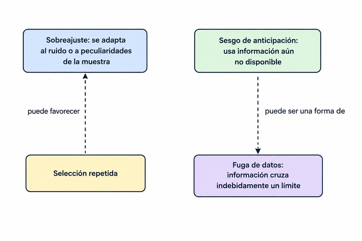
In practice, the model is only one part of the test. A strategy’s signals may be calculated correctly while the data timestamp, corporate-action adjustment, execution price, label horizon or parameter-selection process is wrong. Review the research process as a system. The guidance in testing and validating AI trading systems provides the wider testing context; this article focuses on the ways a backtest can accidentally learn from, or peek at, information it should not have.
Why trading models are easy to overfit
Overfitting is a mismatch between flexibility and evidence. A model with enough parameters can fit patterns in a finite sample, whether those patterns represent a durable market relationship or random historical noise. A strategy search has the same issue even when each candidate is simple: try enough entry rules, holding periods, filters, assets and stop settings, and some combination will look unusually good by chance. The winner’s reported performance is then conditional on having won the search. It is not an unbiased estimate of how that candidate would have performed if it had been chosen in advance.
Financial history makes the problem harder to judge. Prices and returns are noisy, market conditions change, and many observations are related to nearby observations. A model may appear to have a large sample because it has thousands of rows, while the number of independent market episodes is much smaller. A strategy tested across many correlated instruments can also seem to have broad evidence when the instruments share the same underlying exposure. A high score is not automatically strong evidence. The data’s structure, the number of choices considered and the way the test was run all affect what the result means.
Machine learning can widen the search because it makes it easy to change features, model classes, hyperparameters and decision thresholds. Human-led research has the same selection risk: a trader may test variations manually, forget failed attempts, then remember only the promising result. The risk grows when researchers repeatedly inspect the “test” period and adjust the model in response. That period has then become part of development, whatever its label in a notebook.
Research on the probability of backtest overfitting describes how selecting the best-performing configuration among many candidates can leave a strategy that ranks poorly on data it did not win on. The paper proposes a method for examining selection risk across candidate strategies. It does not turn a backtest into a guarantee, and its result should not be read as the probability that a live account will lose money. The useful lesson is narrower: the discarded trials matter. A report that shows only the final winner hides part of the evidence needed to judge it.
Look-ahead bias: using information from the future
Look-ahead bias occurs when a simulated decision uses a value that was not yet available at its decision time. The mistake can be obvious, such as using tomorrow’s closing price to decide whether to buy today. More often, it hides in data joins and timestamps. A row may carry the date an event refers to, not the date the event became public. A daily bar may be stamped with the trading date even though its final high, low and close are only known after the session ends.
Suppose a strategy makes a decision at 10:00 a.m. using the day’s closing price, a full-session volume total or a signal calculated from that day’s high and low. The backtest may show trades executed at 10:00, but those values were not yet complete then. The model has been allowed to see the remainder of the session. To test a decision at the close, a closing-price feature may be valid, but the assumed fill must occur after the signal is available, not at a price that could only have been known before it.
Time alignment must include publication and processing delays, not only calendar dates. An economic release labelled “March” may be published in April. An earnings value may refer to a quarter that ended weeks earlier, while the market first received it on the results announcement date. A closing price in one time zone may occur after a decision timestamp in another. If a dataset stores only the event date, it may not contain enough information to simulate when a trader could have acted.
Revisions create a subtler version. Economic statistics, index membership, corporate fundamentals and vendor data can be updated after their first release. A present-day database may show the latest corrected value for a past date, not the vintage that a trader could have seen then. A backtest using the revised series can inherit future information even when every row’s date appears to precede the trade. Historical market research therefore needs point-in-time records, or a clear account of how publication times and revisions were handled. See preparing historical market data for AI trading research for the related data-quality questions.
Data leakage: information crossing the wrong boundary
Data leakage covers more than a feature with an obvious future value. It can happen while creating labels, splitting observations, preprocessing features, selecting variables, choosing a model or calculating performance. The shared feature is that information from outside the permitted training process influences a result that is presented as if it were independent. A pipeline can have a chronological train/test split and still leak information if it performs a global transformation before making that split.
Consider a feature standardised by subtracting the mean and dividing by the standard deviation of the entire dataset. If the test period contributes to those statistics, its distribution has influenced the representation used to train the model. This may not expose the test labels, but it still lets the training process use information from the test period. The remedy is to fit the scaler on the training window, then apply those fixed training statistics to validation or test data. The same rule applies to imputation, feature selection, dimensionality reduction and any transformation that learns values from a sample.
Leakage can also enter through target construction. A label might represent the return over the next five sessions. If observations are randomly split, a training label’s outcome window can overlap with a test period, or adjacent samples can share much of the same future return interval. The model may then be evaluated on outcomes partly represented in its training data. Even with chronological splits, labels near the boundary can reach across it. The test design must account for when each label begins and ends, not just the timestamp assigned to its row.
Another route is feature selection performed once on the full history. If a researcher ranks variables by their relationship with the target using all dates, then uses the selected variables in an earlier training window, the future target outcomes have already influenced the choice. Feature selection belongs inside the training process for each fold. The same applies to threshold selection: if a buy probability cutoff is picked by inspecting test-period results, that period is no longer an untouched evaluation.
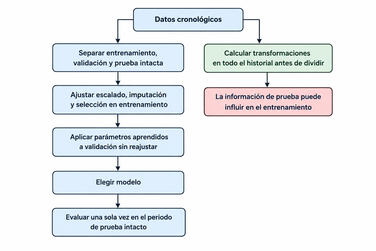
Common failure points in a trading research pipeline
Random splits for time-ordered data
Randomly assigning rows to training and test sets can put later observations in the training set and earlier observations in the test set. The model is then evaluated on the past after learning from the future. The official scikit-learn TimeSeriesSplit documentation notes that ordinary cross-validation methods can train on future data and evaluate on past data when applied to time-ordered observations. Chronological splitting is a better starting point for market data, though it does not solve every overlap, timestamp or selection problem.
Random splitting can also produce an unrealistically easy test if neighbouring rows share information. For example, a rolling volatility feature for one day and the next day may rely on nearly all the same price observations. If one row goes into training and its neighbour goes into testing, the two sets are not independent in the practical sense the researcher may assume. The same issue appears in overlapping forward-return labels. The split must reflect the forecast horizon, feature windows and intended deployment process.
Overlapping labels and insufficient gaps
A simple gap between training and test observations can help when labels span multiple periods, but the correct gap depends on how the target and features are defined. If a label is the return over the next ten trading sessions, observations near a boundary may share outcome days. If a feature uses a long rolling window, its input history can overlap across the boundary as well. Overlap is not always automatically leakage: a live model may legitimately use historical prices that are also used in training. The concern is whether test outcomes, or information unavailable at the prediction time, influence the fitted process.
For a forward-return label, write down the label’s start and end time for each observation. Then make sure no training label uses returns that belong to the evaluation interval, and consider a purge or embargo around the boundary when samples overlap. A generic split setting cannot infer the market meaning of your label. The validation design should be explained in terms of the actual forecast horizon and information flow. Details of training, validation and test sets for financial time series are central to that design.
Global preprocessing and feature selection
Any operation that estimates a value from data must be fitted inside each training fold. This includes scaling, imputing missing values, selecting features, reducing dimensions, calibrating probabilities and learning category encodings. If the operation is calculated once on all dates, later information can seep into earlier folds. A sound pipeline treats preprocessing as part of the model, not as a harmless cleanup step done before validation.
Some transformations use only a fixed formula and do not estimate parameters from the dataset. A lagged return calculated from prior prices can be valid when its timestamp is correctly aligned. But a rolling measure must be shifted if the decision occurs before the bar is complete; otherwise it may use the current bar’s unfinished or future values. A rolling calculation can be leak-free in one trading schedule and invalid in another. State when each feature is computed and when the trade could be submitted.
Survivorship and historical universe errors
A stock universe built from today’s listed companies excludes firms that failed, merged or were delisted in the past. A strategy tested on that surviving set may avoid some historical losers by construction. Similarly, using current index constituents in a past-period test can include companies before they joined the index and omit companies that later left. This is not always described as look-ahead bias in a narrow sense, but it is a point-in-time universe error that can make a historical test unrepresentative.
Trading universes also change through ticker changes, mergers, delistings and listing dates. If the research omits delisted securities or handles delisting returns inconsistently, reported results may be distorted. A proper audit records which securities were eligible at each decision time and how the test handles corporate actions, delisting events and missing observations. The data should reflect what a strategy could have selected then, not only what remains easy to download now.
Execution prices that cannot be obtained
A signal based on a closing price cannot generally be assumed to transact at that same closing price unless the order process and market mechanics make that execution plausible. If the model only knows the final close after the closing auction, filling at that close without an executable order submitted in time is a timing error. Similarly, a signal based on a bar’s high or low cannot assume a fill at that extreme unless the order was live and the market traded there after the order became active.
Execution assumptions are not just a cost adjustment. They can expose a hidden timing mismatch between signal generation and the assumed order. Use a feasible next price, auction process or execution model that matches the strategy’s actual decision schedule, then include fees, spread and slippage. A test can avoid look-ahead and still be unrealistic if it assumes fills that would not have been available. The related guide on including fees, spreads, slippage and financing costs in backtests covers those separate performance distortions.
Language models and information in training data
Text-based strategies face an additional timing problem: a model may have been trained on material published after the historical article being evaluated. Asking a current language model to interpret an old headline does not recreate what a model could have known at the time. Its training data may contain later news about the company, its subsequent performance or commentary that was not yet public when the headline appeared.
A study by Paul Glasserman and Caden Lin examined this issue in GPT-based sentiment analysis of financial news headlines. It distinguishes possible knowledge of subsequent events from a separate effect in which general company knowledge influences the model’s interpretation. The distinction matters: removing company identifiers can help probe some information effects, but it does not certify a model as point-in-time. See the paper on look-ahead bias in GPT sentiment analysis for its method and findings. For a historical test, record the model version, training cutoff if known, prompt, source text and retrieval date; do not assume that an old input makes a current model historically uninformed.
How overfitting sneaks in through repeated testing
Backtest overfitting is often a research-process problem. A researcher might start with a trend strategy, inspect results, add a volatility filter, change the lookback, test another market and adjust the exit. Each change can be reasonable on its own. But if every choice is made after looking at the same historical results, the final model has been selected using that history many times. Keeping a nominal test period while repeatedly consulting its score does not preserve its independence.
The number of trials is broader than the number of trained model files. Count manual parameter changes, feature sets, assets, date ranges, label definitions, benchmark choices, risk rules and strategy variants that influenced the final decision. Also record failed trials. A team that runs fifty experiments and publishes the best one has a different selection process from a team that specified one model and tested it once, even if the winner’s Sharpe ratio is identical.
Keeping a research log is a practical defence. Record the hypothesis, data window, candidate settings, selection metric, result and decision for each material experiment. Store code and configuration versions so that the final report can be reproduced. This record will not prevent overfitting by itself, but it makes hidden search visible. A result that only survives when the researcher forgets the other attempts is not strong evidence.
A disciplined validation design
1. Write down the decision timeline
Before fitting the model, specify when each prediction is made, what information is available at that moment, when an order could be sent and how the label is calculated. Use a concrete timeline, not vague words such as “daily.” A system that calculates after the close and trades at the next open has different valid inputs from a system that trades during the session. This step catches many timing errors before a model is involved.
For every feature, document its source, event time, publication or availability time, transformation and any delay. For the target, note the exact start and end of the return window. Include time zone, exchange calendar and treatment of non-trading days. Where a source revises historical values, retain the point-in-time vintage if possible. When a vendor cannot provide it, disclose the limitation and avoid claiming that a revised series perfectly represents what traders knew at the time.
2. Separate model fitting, model selection and final evaluation
Use chronological training and validation windows to fit parameters and choose among candidate models. Keep a later test period for a final check, and do not use its result to revise the model and still call it untouched. If the test result leads to another feature or threshold change, that period has become part of development. A new independent evaluation then requires data not used to make that change, or a clear statement that the reported test is no longer an independent estimate.
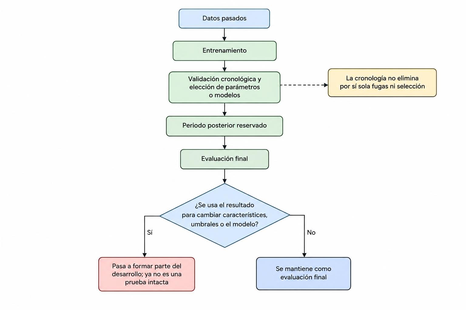
Rolling or expanding walk-forward tests can show how a process behaves as training data and market conditions change. They are useful when they mimic the intended retraining schedule: fit on past data, predict the next period, then move the window forward. They do not guarantee independence if the researcher tunes the system after inspecting all fold results. Learn more about walk-forward testing and out-of-sample evaluation before treating a sequence of folds as a final verdict.
3. Put preprocessing inside each fold
Build a pipeline that fits each learned preprocessing step using only that fold’s training observations. Apply the resulting transformation to validation data without refitting it on the validation observations. After model and settings are chosen, fit the process on the full development window and evaluate once on the untouched test window. This structure reduces the chance that scaling, imputation or feature selection will reveal anything about later observations.
Test the pipeline with a deliberately simple baseline. For example, compare against a model that uses only a small set of lagged price or return features, or a fixed rule selected before examining the final test. A complex model that barely improves on a naïve benchmark may not justify its extra flexibility. Benchmark selection itself should be reasonable and recorded; choosing a weak comparator after seeing the results only creates another route to a flattering chart.
4. Match the split to the task
A single chronological holdout is easy to understand but can be sensitive to the particular market period it contains. Multiple walk-forward folds provide a view across different periods, while still respecting chronology. The folds should have a clear purpose: development, model selection or reporting robustness. Do not average every fold into one number and hide a severe failure in one important regime.
For overlapping labels, use a split and any purge or gap that reflects the target’s outcome window. For assets that share dates and common exposures, split by time across the panel rather than scattering same-date assets randomly between train and test. Otherwise the model may learn broad market conditions from one group of assets and be evaluated on another group experiencing those same conditions. The right design depends on whether the intended use is predicting later dates, new assets, or both.
Checks that expose suspicious results
- Audit timestamps. Pick a sample of trades and trace each feature back to the value available before the decision. Check release time, bar completion, time zone and any publication lag.
- Rebuild the feature pipeline by date. Confirm that rolling features use only permitted observations, and that learned transformations are fitted separately inside training folds.
- Inspect boundary observations. Verify that forward labels, holding periods and rolling windows do not carry test outcomes into training labels or training decisions.
- Compare the full search to the reported strategy. Count every tried configuration, including manual iterations and discarded variants. Keep this history with the report.
- Use a deliberately delayed signal. Shift signals or execution by one period as a diagnostic. A dramatic collapse can indicate fragile timing or unrealistic fills, though it is not proof of leakage on its own.
- Test simpler alternatives. Compare a model with fewer features and parameters. If complexity adds no stable advantage across folds, the added fit may be noise.
- Review concentrated returns. Check whether a small number of trades, instruments or dates account for most gains. A strong headline metric can hide dependence on one exceptional episode.
- Run the process on new data once. Freeze features, parameters, thresholds and reporting rules first. If results are inspected and then used to revise the model, the new data has joined development.
These checks answer different questions, and no one score replaces them all. Performance measures such as Sharpe ratio, drawdown and turnover describe the tested result; they do not establish that the data flow was valid. A strategy may score well while leaking, or score poorly despite a clean test because the underlying hypothesis has no edge. Review performance alongside the research design, using measures beyond win rate rather than relying on one attractive metric.
A hypothetical example: the “perfect” earnings model
Suppose a researcher trains a model to buy stocks after positive earnings surprises. The historical dataset contains quarterly earnings values, announcement dates and daily stock prices. The first backtest looks unusually strong. On inspection, the earnings table records the fiscal quarter end as its date, while the final earnings figure was released several weeks later. The model’s feature join therefore assigns the eventual figure to an earlier date. A simulated trade appears to anticipate an announcement that had not occurred.
The researcher corrects the join to use the publication timestamp, and performance falls. A second issue remains: the surprise score was standardised over the full sample before the time split. That lets the later period influence the training transformation. The team moves scaling inside each fold, then finds that one earnings variable was selected using its relationship with returns across all years. The variable selection is now repeated within each training window. Each fix removes one source of leakage; none requires assuming the original model had no possible predictive value.
Finally, the team notices that dozens of announcement filters, holding periods and thresholds were tried. The best result was selected from that search. The final untouched period has already been viewed several times during development, so it cannot honestly be presented as a pristine test. The team freezes the research process, logs the trials, chooses a simpler specification using development data and waits for genuinely new observations to evaluate it. This example is hypothetical, but the sequence illustrates why data timing, preprocessing and repeated selection need separate audits.
What a backtest can and cannot establish
A carefully designed historical test can show how a defined process would have behaved under stated data and execution assumptions. It can reveal obvious implementation mistakes, compare candidate rules and expose instability across time windows. It cannot prove that a future market will repeat a historical relationship, that available data are free of every revision issue, or that a model will behave as expected once deployed. Those limits remain even when no leakage is found.
Keep claims proportional to the evidence. Describe the data source and coverage, how timestamps were aligned, how the universe was constructed, how many configurations were tried, how the validation periods were chosen and what execution costs were included. Report weak periods as well as strong ones. A clear account lets another person distinguish a potentially useful signal from a strategy that simply fitted a convenient patch of history.
Before moving from research to simulated or live use, freeze the model and define monitoring rules. Paper trading can reveal data-feed delays, order timing mismatches and operational failures that a historical backtest does not capture, though simulated fills still cannot reproduce every live condition. See what paper trading can establish and how model drift and performance decay affect a trading system when planning the next evaluation stage.