A trading model does not have to name tomorrow’s closing price to produce a useful forecast. It can estimate a future return, the chance of an increase, or the likelihood that a return will fall inside a defined range. Those are different prediction targets, and each answers a different question. A model that predicts price asks, “What might the asset be worth?” A model that predicts returns asks, “How much might an investor gain or lose over a period?” A directional model asks, “Which side of a threshold is more likely?” A probability model adds, “How confident should we be in that estimate?”
Choosing among them changes how the model is trained, evaluated, and used. A close price forecast can look accurate because prices move gradually, even when it provides little information about the next move. A direction forecast can be right often but still lose money if its wrong calls are costly. A return forecast can estimate the average outcome while saying little about the risk around it. The right target begins with the decision the model is meant to support: ranking assets, setting an entry filter, sizing a position, or estimating a range of possible outcomes.
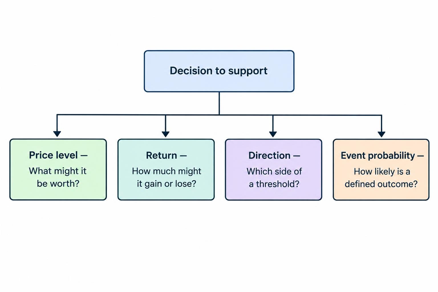
Start with the decision, then define the target
Before selecting a model or metric, write down what action its output may change. A portfolio screen might need to rank securities by expected return over the next month. A short term system might need to estimate the chance that price rises enough to cover trading costs before a stop is reached. A risk process might care more about the probability of a large loss than about the average forecast. Those tasks need different labels. “Predict the market” is not a usable target; it leaves the outcome, horizon, and decision rule undefined.
For every target, define the asset, forecast time, holding horizon, price or return convention, and outcome threshold. Specify whether the forecast uses a closing price, a midpoint, or an executable price, and whether dividends, funding, or other cash flows are included. A forecast made after the close cannot use information that becomes available later that day. This sounds obvious, yet timestamp mismatches can quietly make a model appear prescient. The data construction should match the actual point at which a decision could have been made, as covered in this guide to preparing historical market data for AI research.
Why predicting price levels can mislead
A price is a level. For a stock trading near $100, a forecast of $101 may be close in absolute terms. For a stock trading near $10, the same dollar error is enormous in percentage terms. Even for one asset, a model that predicts tomorrow’s close as today’s close can score well on a conventional error metric when daily changes are small relative to the price level. Yet that model may provide no actionable signal about whether to buy, sell, or wait.
Price levels also tend to scale over time. A model can produce a low average error by tracking that broad scale while missing the changes that matter to a trading decision. Comparing raw price errors across securities is especially awkward because a one dollar error does not carry the same meaning for every instrument. A percentage error or normalized measure can improve comparability, but it does not fix a target that fails to match the intended decision. If the purpose is to estimate performance over a holding period, returns usually express that outcome more directly than future price levels.
Price forecasts still have legitimate uses. They may support an expected price range, a valuation process, or planning around a known cash obligation. If a future price estimate is genuinely required, compare it with a simple baseline such as carrying forward the latest available price, and report errors in a scale-aware way. Do not assume that an impressive-looking chart proves the model can forecast short term market moves. The forecast may be following the level rather than detecting a useful change.
Predicting returns: size as well as direction
A return measures the change in value over a chosen interval. A simple return from time t to time t+h is the future price divided by the current price, minus one. A log return is the logarithm of that ratio. The choice matters less than using one definition consistently and documenting how distributions, contract rolls, and other relevant adjustments are handled.
Returns make it easier to compare outcomes across assets with different price levels. A 2% gain has a comparable percentage meaning whether the instrument trades at $20 or $200. A return target also fits naturally with portfolio performance and many risk calculations. Empirical finance research commonly evaluates forecasts of returns, including machine learning studies that test whether characteristics help predict future stock returns rather than relying solely on price-level accuracy. The published study of machine learning in empirical asset pricing is one example of research framed around return prediction.
A regression model trained on returns typically estimates a conditional average: given the inputs, what return does the model expect over the chosen horizon? That estimate can be useful for ranking opportunities or comparing a forecast with an estimated cost. But an average hides the distribution. A predicted return of 0.3% could reflect many modest positive outcomes, or a mix of frequent small losses and rare large gains. The same average can therefore describe very different risks.
Return targets also require a clear horizon. Predicting a one day return is not the same task as predicting a one month return. Longer holding periods can produce greater variation in outcomes, and returns measured over overlapping periods share observations. A daily model that predicts the next 20 trading days may generate a new label each day, with most labels covering many of the same sessions. Those observations are not independent just because the rows have different dates. Choose evaluation methods that respect the time structure and label overlap; the guide to training, validation, and test sets for financial time series covers the separation problem.
Predicting direction: a simpler question with a trade off
A directional target converts a future return into a category. A basic label might be “up” if the return is above zero and “down” otherwise. This simplifies the task: the model no longer has to estimate the size of the move. That can be useful when the intended decision depends on direction alone, or when precise return estimates are too unstable for the use case. It also discards information. A forecast of a 0.01% rise and a forecast of a 5% rise receive the same positive label.
Accuracy is an easy metric to understand, but it can conceal weaknesses. If positive outcomes are common, a model that always predicts “up” may look accurate without separating better opportunities from worse ones. A direction model can also be right more often than it is wrong and still lose money if its losing calls are larger than its winners. Conversely, a model with modest accuracy may be useful if its strongest positive forecasts tend to precede sufficiently large gains. The trading result depends on the sizes and costs of outcomes, not a hit rate in isolation.
The threshold defining “up” is part of the target, not a harmless technical setting. A zero return threshold labels tiny increases as wins even if they would not cover the spread, fees, or slippage. A threshold above estimated costs may better match a particular trade, but cost estimates can vary by instrument, order type, and market conditions. If the target says “positive return,” do not later present it as “profitable trade” unless costs and execution assumptions are built into the definition. For testing decisions under realistic costs, see how fees, spreads, slippage, and financing affect backtests.
Predicting probabilities: confidence with a defined meaning
A classifier can output a probability rather than only a class. For example, it might estimate a 60% chance that the next five day return exceeds a defined threshold. The threshold and horizon must be stated: “60% chance of a rise” is incomplete if “rise” could mean any positive price change, a 1% gain, or a return greater than estimated trading costs. A probability is useful only when it refers to a well-defined event and a particular forecast period.
Probabilities provide more detail than a hard up or down label. A trading rule could treat forecasts near 51% as weak, while giving more attention to forecasts near 70%, subject to the expected payoff and risk. This does not mean the model is correct 70% of the time on every individual call. It means that, if forecasts assigned similar probabilities are reliable over a sufficiently large and relevant sample, the event should occur about that often. A probability is a statement about a group of comparable forecasts, not a promise about the next trade.
This property is called calibration. To inspect it, group forecasts into probability bands and compare the average forecast with the observed event frequency in each band. If forecasts near 70% are followed by the event only about half the time, the model is overconfident in that region. A reliability diagram can show this pattern. Calibration is distinct from discrimination: a model can rank higher probability cases above lower probability ones but systematically overstate the probabilities. Technical documentation for probability calibration tools and reliability curves describes common ways to assess or adjust classifier probabilities.
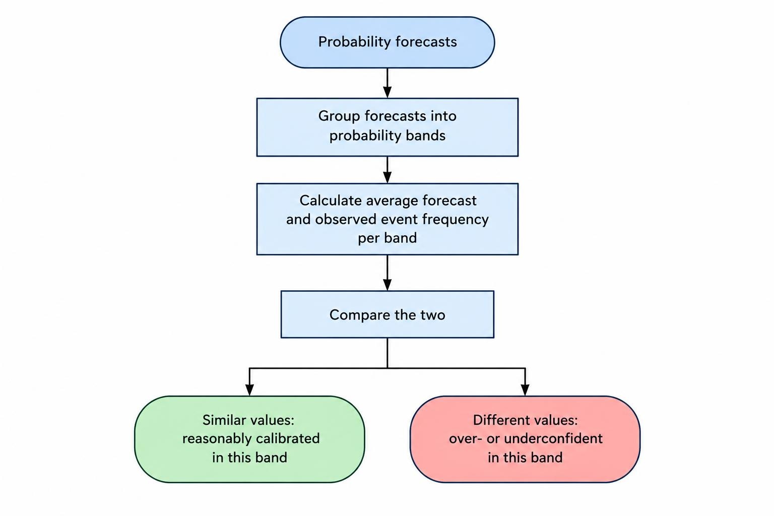
Calibration can also deteriorate when market conditions change. A probability model trained on one period may become too confident or too cautious in another. Recalibrating a model is not a free repair: the adjustment must be fitted on data separate from the final evaluation period, and it should be tested using a time-aware process. Calibration does not establish that a forecast is profitable, either. It tells you whether probabilities correspond reasonably to observed frequencies; the economic value still depends on payoff sizes, costs, position sizing, and risk limits.
Choose the target that matches the question
| Target | What it predicts | Useful evaluation | Main limitation |
|---|---|---|---|
| Price level | A future quoted or adjusted price | MAE or RMSE against a persistence baseline | Can look accurate by tracking the level while missing useful changes |
| Return | Magnitude and sign of the change over a horizon | Error versus a simple return forecast; portfolio or ranking tests where relevant | Large unusual moves can dominate errors; averages conceal uncertainty |
| Direction | Whether return crosses a threshold | Balanced accuracy, precision, recall, or a probability score | Discards move size; accuracy alone says little about profit |
| Event probability | Chance that a defined outcome occurs | Log loss or Brier score, calibration, and discrimination | A calibrated probability is not automatically a profitable signal |
| Return distribution or quantiles | A range or selected points in the possible return distribution | Quantile loss, interval coverage, and decision specific evaluation | More informative outputs can be harder to estimate reliably |
The table is a guide, not a rule that each task needs one target only. A model may estimate both expected return and the probability of crossing a loss threshold. The outputs should still be evaluated separately. A forecast can estimate the mean well while poorly estimating tail risk, or rank opportunities well while being poorly calibrated. Keep the purpose of each output clear, and avoid collapsing distinct questions into a single performance number. Additional measures and their limits are discussed in trading performance metrics beyond win rate.
Three common probability targets
Binary event probability
A binary target defines one event, such as whether the return over the next ten sessions exceeds 1%. The model estimates the probability that the event occurs. This is straightforward to communicate and can support a rule that compares the forecast with a decision threshold. However, the event says nothing about what happens when it does not occur. Returns below 1% could be small gains, flat results, or severe losses. Consider whether the event definition preserves the distinction that matters to the decision.
Up, flat, or down probabilities
A three class target separates returns into positive, near zero, and negative outcomes. The flat band can prevent tiny price fluctuations from being treated as meaningful signals. The boundaries should be chosen before final testing and should have a rationale connected to the trading horizon, market noise, or expected costs. If the middle band is set after inspecting the test results, the apparent performance can be inflated by tuning the target to the sample.
The three probabilities should sum to one. A model might assign 45% to an upward outcome, 30% to flat, and 25% to a downward outcome. That does not mean the expected return is positive: a 25% chance of a sharp loss could outweigh a 45% chance of a small gain. Class probabilities describe categories; they do not automatically state the average payoff inside each category.
Quantiles and ranges
Quantile forecasts estimate points in the outcome distribution, such as a lower, middle, and upper return level. They can answer questions that a single expected return cannot, including how wide the plausible range may be or how severe a downside scenario could be. An interval forecast should be checked for both coverage and width. A very wide range can contain most observed outcomes and still be unhelpful; a narrow range that misses often is falsely precise.
Quantiles are not the same thing as a complete probability distribution. A few predicted percentiles do not describe every possible outcome, and their ordering should make sense. If the model’s estimated lower quantile exceeds its upper quantile, the forecast is internally inconsistent. Distribution forecasts need their own tests, rather than borrowing a directional model’s accuracy score.
How to evaluate each type of forecast
For price or return regression, mean absolute error (MAE) reports average absolute error and is less sensitive to very large misses than root mean squared error (RMSE). RMSE penalizes large errors more heavily. Neither metric tells you whether a forecast improves on a basic alternative. Compare the model with a simple benchmark, such as no expected return, a historical average calculated using past data only, or a straightforward rule relevant to the task. A complex model should earn its place by adding value over that baseline.
For directional classification, report more than raw accuracy. Balanced accuracy gives the two classes more equal weight when their frequencies differ. Precision asks how often positive calls are positive; recall asks how many positive outcomes the model identifies. These statistics still ignore the size of returns and trading costs, so they describe classification quality, not net performance. If the system uses probabilities, evaluate the probability forecasts as probabilities rather than converting them to labels too early.
For probabilities, the Brier score measures squared differences between forecast probabilities and binary outcomes; log loss penalizes forecasts that assign very low probability to events that occur. Lower scores are better when measured on the same target and evaluation sample. These scores combine more than calibration alone, so pair them with a calibration plot and a measure of how well the model distinguishes cases with different outcomes. Choose the test set and scoring procedure before comparing many candidate models.
For a trading strategy, forecast quality and trading performance are related but not interchangeable. A model can improve prediction error slightly without changing the decisions a strategy makes. Another model may have only a small statistical advantage yet improve ranking among a group of assets. Test the whole decision process with realistic assumptions, compare it against relevant benchmarks, and account for the number of variants tried. Repeatedly adjusting target thresholds or model settings until one backtest shines can select noise; research on the probability of backtest overfitting examines this selection problem.
Build a target without leaking the future
Every target is defined using a future outcome, but every model input must be available at the forecast time. If the label uses the return from tomorrow’s open to the close, features must not include tomorrow’s opening price unless the decision is made after that price is known. Corporate action adjustments, revised data, delayed news timestamps, and missing market sessions can create subtle timing errors. Record how each feature and label is timestamped, then check that the model could have generated its forecast in real time.
Keep the target definition fixed during final evaluation. If you test several thresholds, horizons, or asset universes, log those trials. Otherwise, the “best” target may simply be the one that happened to fit the historical sample. Use chronological evaluation: train on earlier data, tune using a later period, and reserve a still later period for the final test. For labels that overlap across adjacent dates, ensure that information from a test outcome does not leak into training labels nearby. The companion guides on overfitting and data leakage and walk forward testing address these validation risks.
Before building a sophisticated model, make a compact target specification. It should state the forecast time, horizon, outcome formula, threshold or class boundaries, treatment of costs and distributions, baseline, evaluation metrics, and data split. A target that cannot be explained in a sentence or two is often too vague to test cleanly. The specification also helps prevent a common research slip: changing the question after seeing results, then presenting the final version as if it had been chosen in advance.
Turning forecasts into decisions
Suppose a model estimates a 60% chance of a gain over the next session. That probability alone does not say whether a trade is attractive. The potential gain if correct, potential loss if wrong, and estimated execution costs all matter. A simple expected value calculation combines outcome probabilities with the payoffs associated with each outcome, then subtracts relevant costs. If the winning outcomes are small and losing outcomes large, a 60% hit rate can still imply an unattractive trade.
Similarly, a predicted return of 0.4% is not a guaranteed gain of that size. It is an estimate tied to a target definition and historical testing process. A trader might use it as one input in a screen, or combine it with a risk estimate and a rule that rejects forecasts too close to estimated costs. The decision rule should be tested separately from the forecasting model. Selecting a probability threshold because it maximizes returns on the same data used to fit the model invites overfitting.
A practical workflow is to begin with the narrowest target that answers the decision, compare it with a simple baseline, and then add complexity only when it improves out of sample results. If the question concerns ranking assets, assess ranking quality. If it concerns the likelihood of crossing a risk threshold, forecast that event and check calibration. If it concerns how much a position might gain or lose, model returns and examine the error distribution. Keeping target, metric, and decision aligned makes the results easier to interpret—and much harder to dress up as a forecast the model never made.